Home / icechunk-python / virtual

Virtual Datasets

While Icechunk works wonderfully with native chunks managed by Zarr, there is lots of archival data out there in other formats already. To interoperate with such data, Icechunk supports "Virtual" chunks, where any number of chunks in a given dataset may reference external data in existing archival formats, such as netCDF, HDF, GRIB, or TIFF. Virtual chunks are loaded directly from the original source without copying or modifying the original achival data files. This enables Icechunk to manage large datasets from existing data without needing that data to be in Zarr format already.

To create virtual Icechunk datasets with Python, the community utilizes the kerchunk and VirtualiZarr packages.

kerchunk allows scanning the metadata of existing data files to extract virtual references. It also provides methods to combine these references into larger virtual datasets, which can be exported to it's reference format.

VirtualiZarr lets users ingest existing data files into virtual datasets using various different tools under the hood, including kerchunk, xarray, zarr, and now icechunk. It does so by creating virtual references to existing data that can be combined and manipulated to create larger virtual datasets using xarray. These datasets can then be exported to kerchunk reference format or to an Icechunk store, without ever copying or moving the existing data files.

Creating a virtual dataset with VirtualiZarr

We are going to create a virtual dataset pointing to all of the OISST data for August 2024. This data is distributed publicly as netCDF files on AWS S3, with one netCDF file containing the Sea Surface Temperature (SST) data for each day of the month. We are going to use VirtualiZarr to combine all of these files into a single virtual dataset spanning the entire month, then write that dataset to Icechunk for use in analysis.

Before we get started, we also need to install fsspec and s3fs for working with data on s3.

pip install fsspec s3fs

First, we need to find all of the files we are interested in, we will do this with fsspec using a glob expression to find every netcdf file in the August 2024 folder in the bucket:

import fsspec

fs = fsspec.filesystem('s3')

oisst_files = fs.glob('s3://noaa-cdr-sea-surface-temp-optimum-interpolation-pds/data/v2.1/avhrr/202408/oisst-avhrr-v02r01.*.nc')

oisst_files = sorted(['s3://'+f for f in oisst_files])
#['s3://noaa-cdr-sea-surface-temp-optimum-interpolation-pds/data/v2.1/avhrr/201001/oisst-avhrr-v02r01.20100101.nc',
# 's3://noaa-cdr-sea-surface-temp-optimum-interpolation-pds/data/v2.1/avhrr/201001/oisst-avhrr-v02r01.20100102.nc',
# 's3://noaa-cdr-sea-surface-temp-optimum-interpolation-pds/data/v2.1/avhrr/201001/oisst-avhrr-v02r01.20100103.nc',
# 's3://noaa-cdr-sea-surface-temp-optimum-interpolation-pds/data/v2.1/avhrr/201001/oisst-avhrr-v02r01.20100104.nc',
#...
#]

Now that we have the filenames of the data we need, we can create virtual datasets with VirtualiZarr. This may take a minute.

from virtualizarr import open_virtual_dataset

virtual_datasets =[
    open_virtual_dataset(url, indexes={})
    for url in oisst_files
]

We can now use xarray to combine these virtual datasets into one large virtual dataset (For more details on this operation see VirtualiZarr's documentation). We know that each of our files share the same structure but with a different date. So we are going to concatenate these datasets on the time dimension.

import xarray as xr

virtual_ds = xr.concat(
    virtual_datasets, 
    dim='time', 
    coords='minimal', 
    compat='override', 
    combine_attrs='override'
)

#<xarray.Dataset> Size: 257MB
#Dimensions:  (time: 31, zlev: 1, lat: 720, lon: 1440)
#Coordinates:
#    time     (time) float32 124B ManifestArray<shape=(31,), dtype=float32, ch...
#    lat      (lat) float32 3kB ManifestArray<shape=(720,), dtype=float32, chu...
#    zlev     (zlev) float32 4B ManifestArray<shape=(1,), dtype=float32, chunk...
#    lon      (lon) float32 6kB ManifestArray<shape=(1440,), dtype=float32, ch...
#Data variables:
#    sst      (time, zlev, lat, lon) int16 64MB ManifestArray<shape=(31, 1, 72...
#    anom     (time, zlev, lat, lon) int16 64MB ManifestArray<shape=(31, 1, 72...
#    ice      (time, zlev, lat, lon) int16 64MB ManifestArray<shape=(31, 1, 72...
#    err      (time, zlev, lat, lon) int16 64MB ManifestArray<shape=(31, 1, 72...

We have a virtual dataset with 31 timestamps! One hint that this worked correctly is that the readout shows the variables and coordinates as ManifestArray instances, the representation that VirtualiZarr uses for virtual arrays. Let's create an Icechunk store to write this dataset to.

from icechunk import IcechunkStore, StorageConfig, StoreConfig, VirtualRefConfig

storage = StorageConfig.s3_from_config(
    bucket='YOUR_BUCKET_HERE',
    prefix='icechunk/oisst',
    region='us-east-1',
    credentials=S3Credentials(
        access_key_id="REPLACE_ME",
        secret_access_key="REPLACE_ME",
        session_token="REPLACE_ME"  
    )
)

store = IcechunkStore.create(
    storage=storage, 
    config=StoreConfig(
        virtual_ref_config=VirtualRefConfig.s3_anonymous(region='us-east-1'),
    )
)

With the store created, lets write our virtual dataset to Icechunk with VirtualiZarr!

from virtualizarr.writers.icechunk import dataset_to_icechunk

dataset_to_icechunk(virtual_ds, store)

The refs are written so lets save our progress by committing to the store.

store.commit()

# 'THAJHTYQABGD2B10D5C0'

Now we can read the dataset from the store using xarray to confirm everything went as expected. xarray reads directly from the Icechunk store because it is a fully compliant zarr Store instance.

ds = xr.open_zarr(
    store, 
    zarr_version=3, 
    consolidated=False, 
    chunks={},
)

#<xarray.Dataset> Size: 1GB
#Dimensions:  (lon: 1440, time: 31, zlev: 1, lat: 720)
#Coordinates:
#  * lon      (lon) float32 6kB 0.125 0.375 0.625 0.875 ... 359.4 359.6 359.9
#  * zlev     (zlev) float32 4B 0.0
#  * time     (time) datetime64[ns] 248B 2024-08-01T12:00:00 ... 2024-08-31T12...
#  * lat      (lat) float32 3kB -89.88 -89.62 -89.38 -89.12 ... 89.38 89.62 89.88
#Data variables:
#    sst      (time, zlev, lat, lon) float64 257MB dask.array<chunksize=(1, 1, 720, 1440), meta=np.ndarray>
#    ice      (time, zlev, lat, lon) float64 257MB dask.array<chunksize=(1, 1, 720, 1440), meta=np.ndarray>
#    anom     (time, zlev, lat, lon) float64 257MB dask.array<chunksize=(1, 1, 720, 1440), meta=np.ndarray>
#    err      (time, zlev, lat, lon) float64 257MB dask.array<chunksize=(1, 1, 720, 1440), meta=np.ndarray>

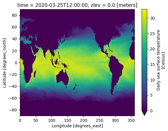
Success! We have created our full dataset with 31 timesteps spanning the month of august, all with virtual references to pre-existing data files in object store. This means we can now version control our dataset, allowing us to update it, and roll it back to a previous version without copying or moving any data from the original files.

Finally, let's make a plot of the sea surface temperature!

ds.sst.isel(time=26, zlev=0).plot(x='lon', y='lat', vmin=0)

Virtual Reference API

While VirtualiZarr is the easiest way to create virtual datasets with Icechunk, the Store API that it uses to create the datasets in Icechunk is public. IcechunkStore contains a set_virtual_ref method that specifies a virtual ref for a specified chunk.

Virtual Reference Storage Support

Currently, Icechunk supports two types of storage for virtual references:

S3 Compatible

References to files accessible via S3 compatible storage.

Example

Here is how we can set the chunk at key c/0 to point to a file on an s3 bucket,mybucket, with the prefix my/data/file.nc:

store.set_virtual_ref('c/0', 's3://mybucket/my/data/file.nc', offset=1000, length=200)

Configuration

S3 virtual references require configuring credential for the store to be able to access the specified s3 bucket. See the configuration docs for instructions.

Local Filesystem

References to files accessible via local filesystem. This requires any file paths to be absolute at this time.

Example

Here is how we can set the chunk at key c/0 to point to a file on my local filesystem located at /path/to/my/file.nc:

store.set_virtual_ref('c/0', 'file:///path/to/my/file.nc', offset=20, length=100)

No extra configuration is necessary for local filesystem references.

Virtual Reference File Format Support

Currently, Icechunk supports HDF5 and netcdf4 files for use in virtual references. See the tracking issue for more info.